When it comes to laser scanning hardware there has been a premium placed upon the increased speed of each successive generation of devices. While there were good reasons to improve upon the “speed” of a Cyrax 2500, this emphasis has swept up point density in the “more is better” paradigm that underlies most sales literature. And in most cases it is; except when it’s not.
If I’m scanning for topographic mapping or volumes, I might only need a point every foot or so but believe me, I’ve never scanned anything that coarsely! Aside from the fact that I want a point cloud dense enough to forego point coding or field attributes, I love looking at (and working with) a beautifully dense point cloud. In fact, as a processor, I wish every cloud I received was photorealistic, with sub-millimeter point spacing! However, if I got my wish I would be broke in short order.
As pretty as those dense clouds are, in a lot of cases they are a waste of money. Before I go into the reasons why, allow me a caveat. There are definitely cases where an incredibly dense point cloud is not only desirable, but necessary. I’m not saying it should never be done, only that it should not be done anywhere near as often as it currently is by general service providers. On some level, we all realize this, but I think that we still overdo the resolution in most cases. Let’s take the Z+F/Leica 6000 series as an example. How many of us routinely scan on the “Ultra High” setting? I would wager that most of us have tried it, but never used it in production. You can collect a point cloud dense enough to model electrical conduit on the “High” setting (which is two below “Ultra High,” for those of you keeping score at home) all while saving almost 20 minutes per scan. We know the “Ultra High” data is usually overkill and that the field time will blow our budget so we don’t use it. To be honest, we could probably get by with the “Medium” resolution setting most days, but the time difference in collection between “Medium” and “High” is so negligible as to make the “High” setting irresistible.
Outside of field costs, the cost of procuring and maintaining storage media can quickly add up as well. However, the real waste comes during processing. The first place this occurs is in the import procedure (if we stick with the Z+F/Leica example). Importing at less than 100 percent density will save you time, but it seems foolish to me if you’ve already realized the cost of collecting the data. The import is an unmanned computer activity, so why not bring it all in? The place to save is after it is in the database, before you start running commands. If it chokes your machine, then reset the point load in the preferences or reduce the point spacing that is displayed to ease the load on your video card.
However, using more data than you need in a command process not only wastes time, it can actually cause some new problems. The best example I can give is in mesh creation. Many projects require the point cloud to be transformed into a mesh. If volumetric computations are to be performed, the mesh will need to be a TIN. When I first started doing this I had a very difficult time creating a mesh that could be verified as a TIN. After a lot of trial and error I learned that unifying the point cloud reduced the errors in the TIN creation. Reducing the point spacing during unification eliminated the errors all together! The greatest difference, however, came when I tried to run the TIN-to-TIN volumetric calculation to determine the displacement volume. When you perform a TIN-to-TIN volumetric displacement calculation the software draws a line (for distance measurement) from each face of the TIN along the Z axis until it strikes the other TIN in the equation. The reduced point spacing reduces the lines that are for the face edges and thus reduces the faces in the TIN, thereby speeding up the calculation. Decimating the mesh further reduces faces and provides a significant increase in the speed of the calculation. I’m talking a drastic reduction, as in reducing a 3-4 hour calculation to a 15-20 minute calculation! The obvious follow up question is, “what about the reduced accuracy?” The answer is the same one you always get in laser scanning, “It depends.”
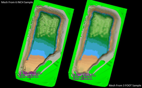
In an example of mining volumes, look at what you are being compared to: a land surveyor with RTK or a total station who is collecting a point every 25 or 50 feet. Between you and him there will be significant volume differences but those differences shrink as the linear distance between point spacing shrinks. Our tests show a volumetric difference of 150-200 cubic yards per acre at a 100′ grid versus  a 3′ grid spacing in a point cloud. However, a 3′ grid versus a 6″ grid only shows a difference  of 20-25 cubic yards per acre. Depending upon the product being measured, you may find that the extra cost of processing to the higher accuracy dataset is more expensive that the actual product being “found” with the denser point cloud.
One last thought concerns the tendency of some operators to attempt to overcome positional errors by raising the point density. No amount of density can replace data from a different angle. Shadows due to occlusion are not altered by the density of the point cloud. It seems obvious but more than once the answer to, “Why don’t we have data on this?” is “I don’t know, I jacked the resolution to make sure we got that area”! Reduce the density of each ScanWorld and add additional ScanWorlds. As long as your control for registration is good, you’ll like the results.
So, once again we see that there are no absolutes in laser scanning. More data is better, except when it’s not. While it is a natural tendency of many of us to be as accurate as possible, the reality is that as the accuracy increases so does the cost. And if there is one issue I hear about from clients more than accuracy, it’s cost.Â