
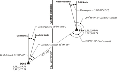
The position of magnetic north is governed by natural forces, but grid north is entirely artificial. In Cartesian coordinate systems, whether known as State Plane, Universal Transverse Mercator, a local assumed system or any other, the direction to north is established by choosing one meridian of longitude. The meridian that is chosen is usually in the middle of the area, the zone, that is covered by the coordinate system. That is why it is frequently known as the central meridian. Thereafter, throughout the system, at all points, grid north is along a line parallel with that central meridian. This arrangement purposely ignores the fact that a different meridian passes through each of the points and all the meridians inevitably converge with one another. Actually, grid north and geodetic north only agree at points along the central meridian, everywhere else in the coordinate system there is an angular difference between the two directions. That angular difference is known as the convergence. East of the central meridian grid north is east of geodetic north and the convergence is positive. West of the central meridian grid north is west of geodetic north and the convergence is negative. The approximate grid azimuth of a line is its geodetic azimuth minus the convergence. Therefore it follows that east of the central meridian the grid azimuth of a line is smaller than its geodetic azimuth. West of the central meridian the grid azimuth of a line is larger than the geodetic azimuth.
The angle between geodetic and grid north, the convergence angle, grows as the point gets further from the central meridian. It also gets larger as the latitude of the point increases. The formula for calculating the convergence in the Transverse Mercator projection is:
γ = (λcm –λ) sin f
where:
- λcm = the longitude of the central meridian
- λ = the longitude through the point
- f = the latitude of the point
The formula for calculating the convergence angle in the Lambert Conic projection is very similar it is:
γ = (λcm –λ) sin fo
where:
- λcm = the longitude of the central meridian
- λ = the longitude through the point
- fo = the latitude of the center of the zone
As an example, here is the calculation of the convergence angle for station Stormy. It is in the Colorado South Zone on a Lambert Conic projection where the longitude of the central meridian is Longitude 105°30’00” West and fo is Latitude 37°50’02.34” North
γ = (λcm –λ) sin φo
γ = (105°30’00”–103º46’35.3195”) sin 37°50’02.34”
γ = (01°43’24.68”) sin 37°50’02.34”
γ = (1°43’24.68”) 0.6133756
γ = +1°03’25.8”
The angle is positive as expected east of the central meridian.
The formula used to convert a geodetic azimuth to a grid azimuth includes the convergence angle, and another element.
grid azimuth = geodetic azimuth – convergence + the second term
Another way of stating the same formula is:
t = α – γ + δ
in which
- t = grid azimuth
- α = geodetic azimuth
- γ = the convergence angle
- δ = the second term
This second tem correction for curvature is sometimes known as t-T, the arc to chord correction and the second term. It is small and pertinent to only the most precise work.